State Utility

Definition

The utility of a state (otherwise known as the state-value ) represents how attractive the state is with respect to the goal. Recall that for each state, the state-value function yields the expected return, if the agent (robot) starts in that state and then follows the policy for all time steps. In mathematical notation, this can be represented as so:

U^{\pi}(s) = E[\sum_{t=0}^{\infty}R(s_t)|\pi , s_0 = s]

The notation used in path planning differs slightly from what you saw in Reinforcement Learning. But the result is identical.

Here,

U^{\pi}(s) represents the utility of a state s ,
E represents the expected value, and
R(s) represents the reward for state s .

The utility of a state is the sum of the rewards that an agent would encounter if it started at that state and followed the policy to the goal.

Calculation

We can break the equation down, to further understand it.

U^{\pi}(s) = E[\sum_{t=0}^{\infty}R(s_t)|\pi , s_0 = s]

Let’s start by breaking up the summation and explicitly adding all states.

U^{\pi}(s) = E[R(s_0) + R(s_1) + R(s_2) + ... \ |\pi , s_0 = s]

Then, we can pull out the first term. The expected reward for the first state is independent of the policy. While the expected reward of all future states (those between the state and the goal) depend on the policy.

U^{\pi}(s) = E[R(s_0)|s_0 = s] + E[R(s_1) + R(s_2) + ... \ |\pi]

Re-arranging the equation results in the following. (Recall that the prime symbol, as on s' , represents the next state - like s_2 would be to s_1 ).

U^{\pi}(s) = R(s) + E[\sum_{t=0}^{\infty}R(s_t)|\pi , s_0 = s']

Ultimately, the result is the following.

U^{\pi}(s) = R(s) + U^{\pi}(s')

As you see here, calculating the utility of a state is an iterative process. It involves all of the states that the agent would visit between the present state and the goal, as dictated by the policy.

As well, it should be clear that the utility of a state depends on the policy. If you change the policy, the utility of each state will change, since the sequence of states that would be visited prior to the goal may change.

Determining the Optimal Policy

Recall that the optimal policy , denoted \pi^* , informs the robot of the best action to take from any state, to maximize the overall reward. That is,

\pi^*(s) = \underset{a}{argmax} E [U^{\pi}(s)]

In a state s , the optimal policy \pi^* will choose the action a that maximizes the utility of s (which, due to its iterative nature, maximizes the utilities of all future states too).

While the math may make it seem intimidating, it’s as easy as looking at the set of actions and choosing the best action for every state. The image below displays the set of all actions once more.

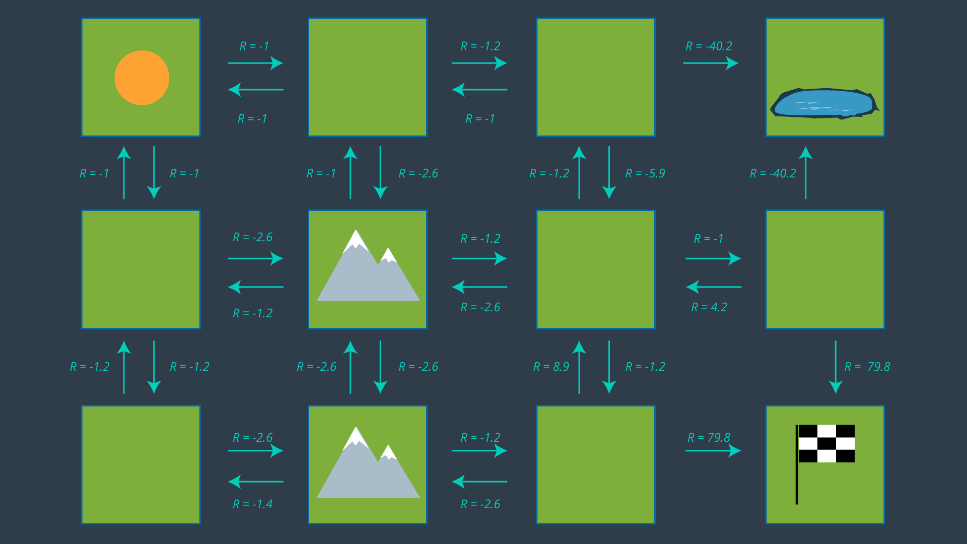
It may not be clear from the get-go which action is optimal for every state, especially for states far away from the goal which have many paths available to them. It’s often helpful to start at the goal and work your way backwards.

If you look at the two cells adjacent to the goal, their best action is trivial - go to the goal! Recall from your learning in RL that the goal state’s utility is 0. This is because if the agent starts at the goal, the task is complete and no reward is received. Thus, the expected reward from either of the goal’s adjacent cells is 79.8. Therefore, the state’s utility is, 79.8 + 0 = 79.8 (based on U^{\pi}(s) = R(s) + U^{\pi}(s') ).

If we look at the lower mountain cell, it is also easy to guess which action should be performed in this state. With an expected reward of -1.2, moving right is going to be much more rewarding than taking any indirect route (up or left). This state will have a utility of -1.2 + 79.8 = 78.6.

Now it's your turn!

Quiz

Can you calculate what would the utility of the state to the right of the center mountain be, if the most rewarding action is chosen?

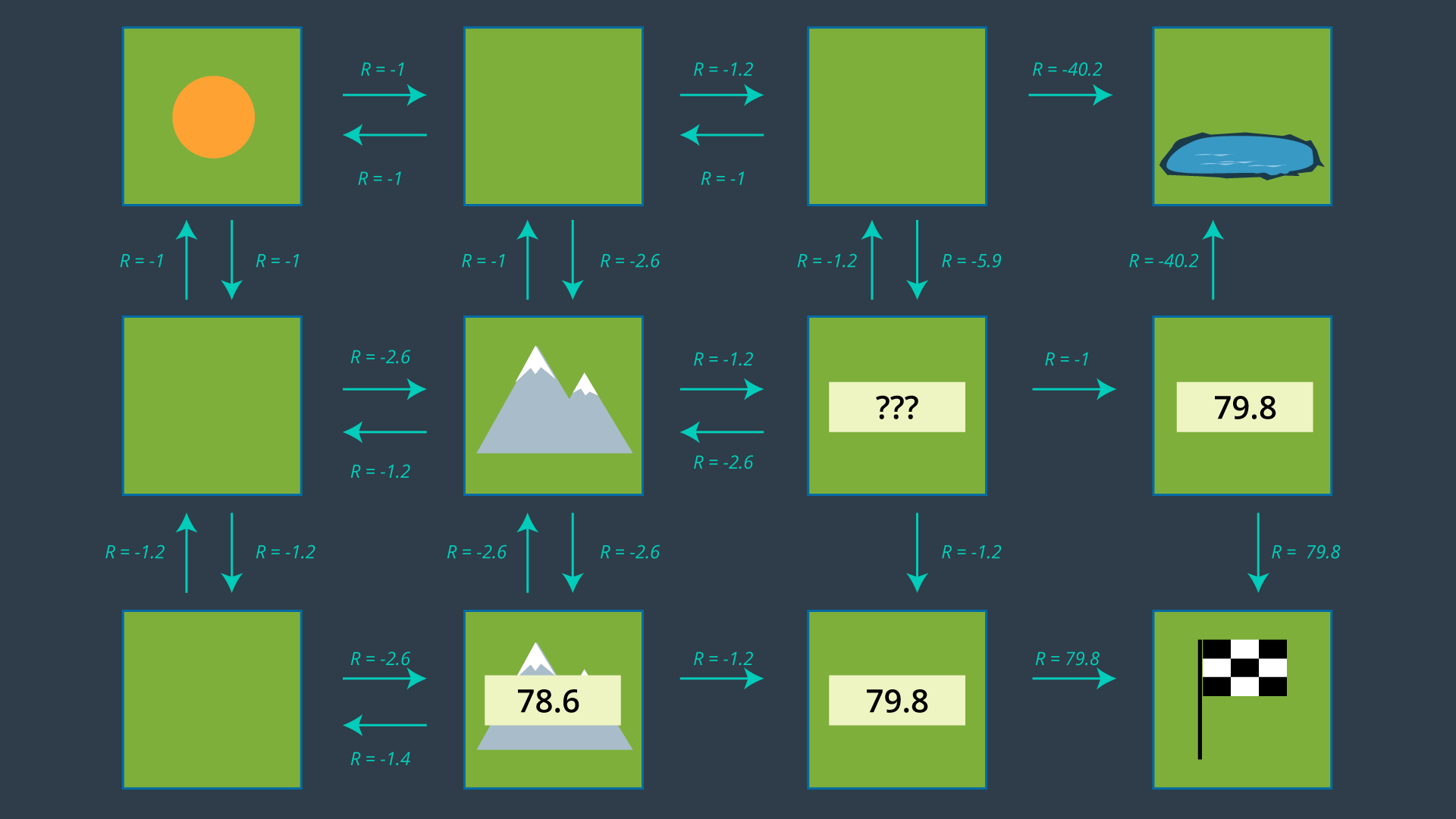
QUESTION:

What is the utility of the state to the right of the center mountain following the optimal policy?

ANSWER:

SOLUTION:

NOTE: The solutions are expressed in RegEx pattern. Udacity uses these patterns to check the given answer

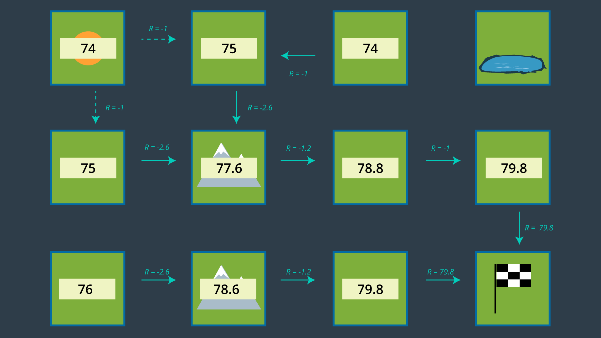
The process of selecting each state’s most rewarding action continues, until every state is mapped to an action. These mappings are precisely what make up the policy.

It is highly suggested that you pause this lesson here, and work out the optimal policy on your own using the action set seen above. Working through the example yourself will give you a better understanding of the challenges that are faced in the process, and will help you remember this content more effectively. When you are done, you can compare your results with the images below.

Applying the Policy

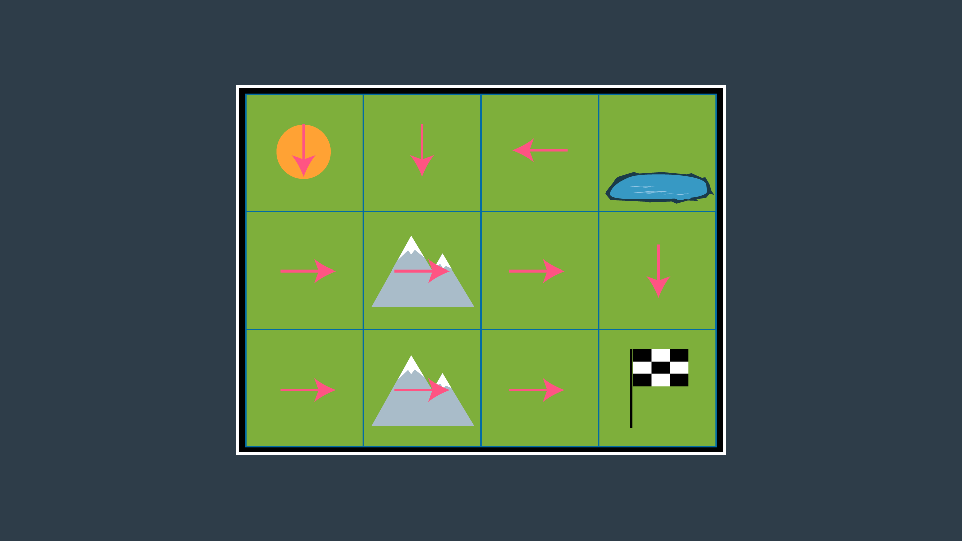
Once this process is complete, the agent (our robot) will be able to make the best path planning decision from every state, and successfully navigate the environment from any start position to the goal. The optimal policy for this environment and this robot is provided below.

The image below that shows the set of actions with just the optimal actions remaining. Note that from the top left cell, the agent could either go down or right, as both options have equal rewards.

Discounting

One simplification that you may have noticed us make, is omit the discounting rate \gamma . In the above example, \gamma = 1 and all future actions were considered to be just as significant as the present action. This was done solely to simplify the example. After all, you have already been introduced to \gamma through the lessons on Reinforcement Learning.

In reality, discounting is often applied in robotic path planning, since the future can be quite uncertain. The complete equation for the utility of a state is provided below:

U^{\pi}(s) = E[\sum_{t=0}^{\infty}\gamma^tR(s_t)|\pi , s_0 = s]